Lid-Driven Cavity CFD Explanation

Introduction to Lid-Driven Cavity Flow

Classic CFD Benchmark Problem

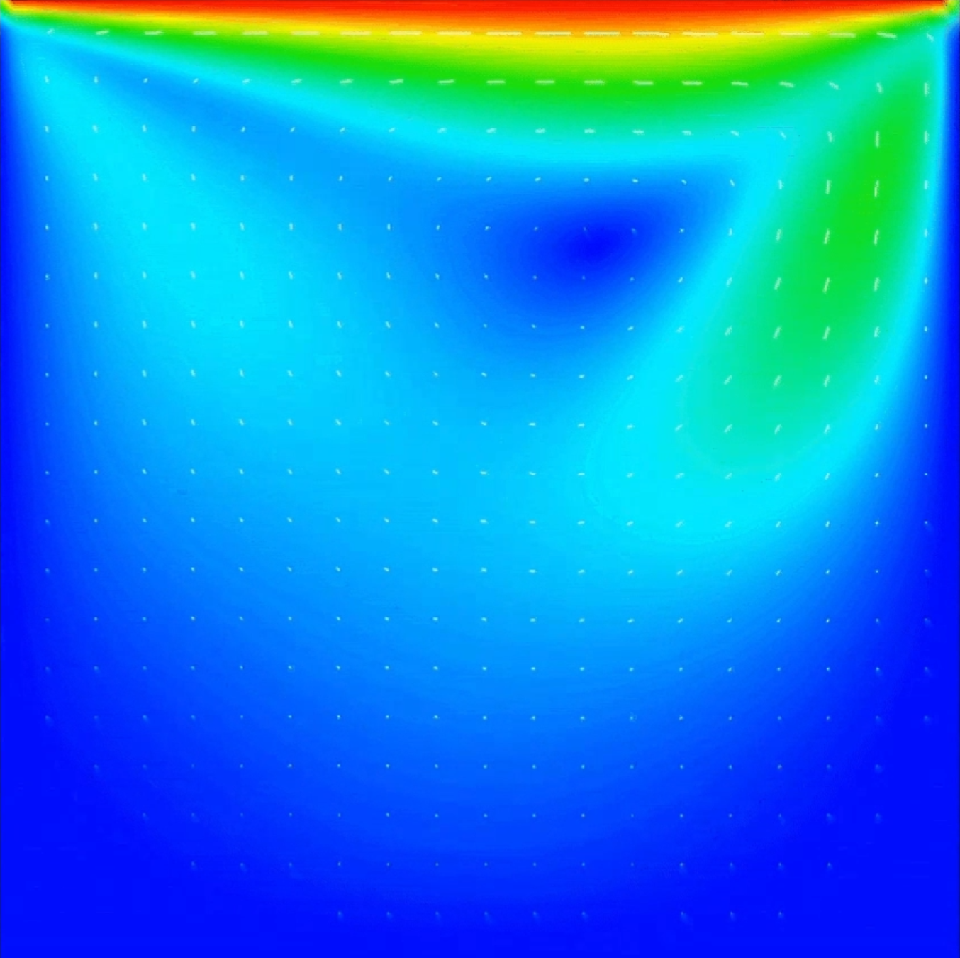
The Lid-Driven Cavity problem is a staple in the CFD community and is a classic problem. The methods required to solve this problem can be easily modified and then applied to more complex applications.

To begin, the Lid-Driven Cavity problem entails a 2-Dimensional square that has a constantly moving top. Think of a conveyor belt. This top is constantly pushing the fluid contained within the square in a certain direction.

Governing Equations

X-momentum equation:

$$\frac{\partial u}{\partial t} + u\,\frac{\partial u}{\partial x} + v\,\frac{\partial u}{\partial y} = -\frac{1}{p}\,\frac{\partial p}{\partial x} + \nu\left(\frac{\partial^2 u}{\partial x^2} + \frac{\partial^2 u}{\partial y^2}\right)$$

Y-momentum equation:

$$\frac{\partial v}{\partial t} + u\,\frac{\partial v}{\partial x} + v\,\frac{\partial v}{\partial y} = -\frac{1}{p}\,\frac{\partial p}{\partial y} + \nu\left(\frac{\partial^2 v}{\partial x^2} + \frac{\partial^2 v}{\partial y^2}\right)$$

These equations are variations of the Navier-Stokes equations. This equation will be broken down into separate parts and solved in the code. More on what this equation actually represents will be explained later on in the solution. For right now, it's just important to understand that we will be using these equations.

Continuity equation:

$$\frac{\partial u}{\partial x} + \frac{\partial v}{\partial y} = 0$$

This equation ensures mass conservation. This applies only to incompressible fluids; water being one such fluid. This is done so that changes in the velocity components are balanced out so that no fluid is accidentally created or lost. This equation does this by ensuring that with an increase/decrease in u along x, it is balanced by a decrease/increase in v along y.

Solution Methodology

Staggered Grid Arrangement

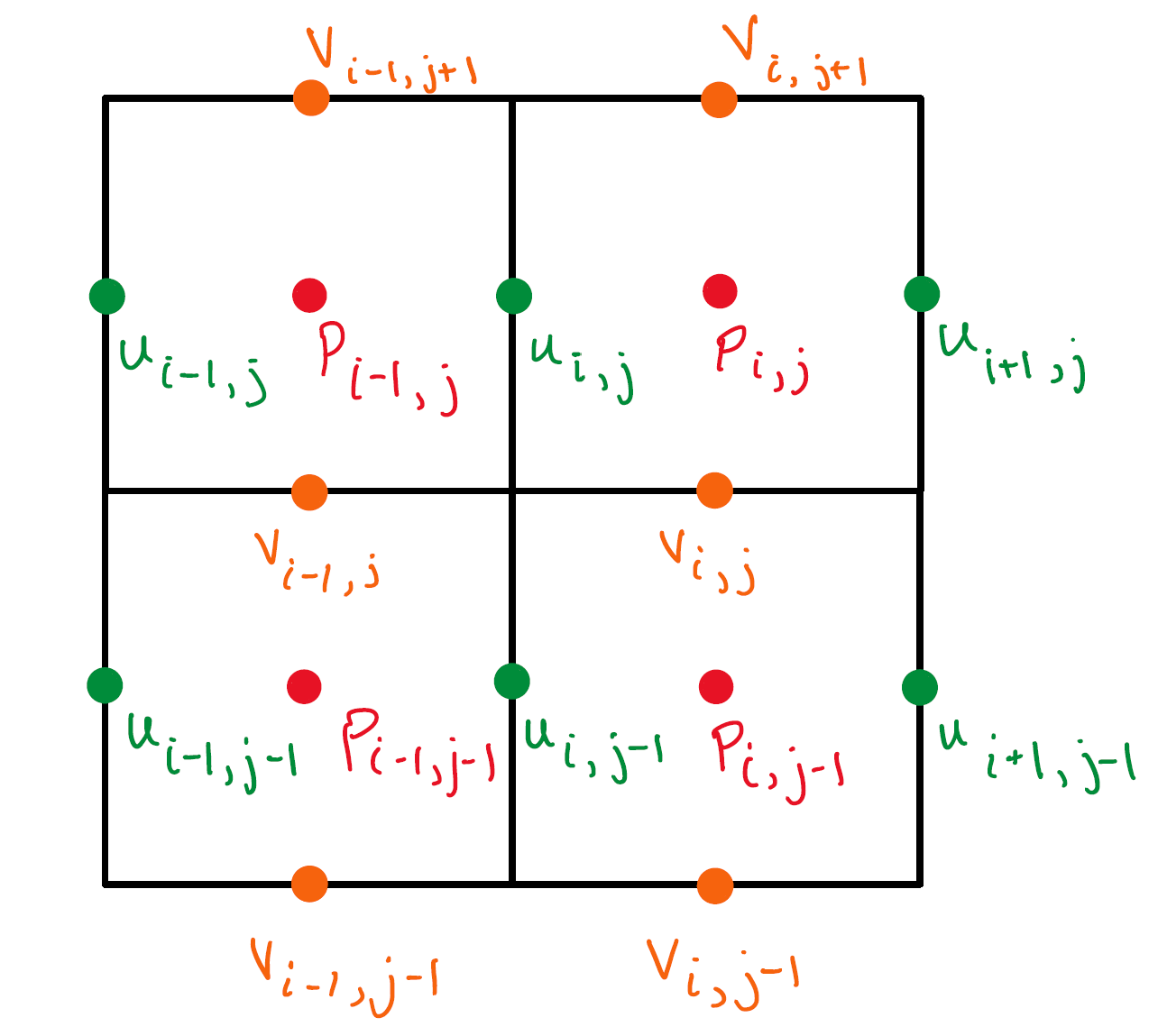
Choose the number of grid cells in x and y directions: these will go by Nx and Ny.

In this grid, the pressure (p) will be stored at the cell centers. Horizontal velocities (u) will be stored at centers of vertical cell faces. Vertical velocities (v) will be stored at centers of horizontal cell faces.

This is done for simpler solutions for momentum equations later on, resulting in a more stable solution.

Finite Difference Approximations

Now it's time to pick apart the formulas from before and use finite difference methods to find numerical approximations for the individual pieces so they can be used in the solver.

Time Derivatives

$$\frac{\partial u}{\partial t} \approx \frac{u_{i+\frac{1}{2},j}^{n+1} - u_{i+\frac{1}{2},j}^{n}}{\Delta t}$$

This is a forward difference approximation in time.

Spatial Derivative (Convection)

$$\left.\frac{\partial u}{\partial x}\right|_{i+\frac{1}{2,j}} \approx \frac{u_{i+1,j} - u_{i,j}}{\Delta x}$$

This is a central difference approximation. It looks like a forward difference approximation but since it is evaluating at a half node, it becomes a central difference approximation.

Spatial Derivative (Diffusion)

$$\left.\frac{\partial^2 u}{\partial x^2}\right|_{i+\frac{1}{2},j} \approx \frac{u_{i+\frac{3}{2},j} - 2\,u_{i+\frac{1}{2},j} + u_{i-\frac{1}{2},j}}{(\Delta x)^2}$$

Another central difference approximation using a second-order central difference formula.

SIMPLE Algorithm Implementation

SIMPLE Method Steps

We use the SIMPLE method, which breaks the problem into smaller steps so that pressure and velocity are computed separately—making sure that the final velocity field obeys the continuity (no fluid compressing or expanding).

Step 1: Initialize the Pressure Field

We start by setting the pressure everywhere to a simple initial guess (often p = 0).

Step 2: Compute Provisional Velocities

Next, we solve the momentum equations (the equations that dictate how fluid moves) using the current pressure field. This gives us provisional velocities, denoted as u* and v*. However, these velocities may not perfectly satisfy the requirement that the fluid's divergence is zero (i.e., they might not be perfectly "balanced" or divergence-free).

Step 3: Derive the Pressure Correction Equation

To fix this, we introduce a correction term, p′, which adjusts our pressure field. This is done by forming the following equation:

$$\nabla^2 p' = \frac{\rho}{\Delta t}\left(\frac{\partial u^*}{\partial x} + \frac{\partial v^*}{\partial y}\right)$$

Let's break this down:

$\nabla^2 p'$: This term represents the "spread" or diffusion of the pressure correction throughout the domain.
$\rho$: The fluid density.
$\Delta t$: The time step over which we is updating our solution.
$\frac{\partial u^*}{\partial x} + \frac{\partial v^*}{\partial y}$: This is the divergence of our provisional velocity field, which shows us how much the current velocities deviate from being divergence-free.

Step 4: Update Pressure and Velocities

Once we have p′, we update our pressure and velocities:

$$p^{n+1} = p^* + \alpha\,p'$$

What does this mean?

p^* is our current (or provisional) pressure.
pⁿ⁺¹ is the updated pressure field.
α is a relaxation factor (typically between 0.3 and 0.7) that helps us smoothly adjust our solution so that it converges faster.

Then, the velocities are updated using:

$$u^{n+1} = u^* - \frac{\Delta t}{\rho}\frac{\partial p'}{\partial x}$$
$$v^{n+1} = v^* - \frac{\Delta t}{\rho}\frac{\partial p'}{\partial y}$$

Boundary Conditions

Enforcing Boundary Conditions

Now we need to apply the boundary conditions. These must be enforced after every iteration:

For the top wall (y = L): set u = U at all nodes and v = 0 (since the lid moves only to the right).
For the bottom and side walls: enforce u = 0 and v = 0. For pressure, apply the Neumann condition (zero normal gradient), meaning there is no change in pressure at the walls.

Implementation Summary

Code Implementation Outline

Finally, the general outline for the code is as follows:

Initialize u, v, and p (start with zero for each).
Simulation Loop:
- Update provisional velocities by solving the momentum equations.
- Solve for the pressure correction p' using the discrete Poisson equation.
- Update the pressure and velocities.
- Check the continuity residual:
  $$\frac{\partial u}{\partial x} + \frac{\partial v}{\partial y} = 0$$
- Explicitly set boundary conditions for u, v, and p at each time step.
- Visualize the movement (this will be done with OpenGL).
- Repeat until the solution converges.